3 Intensity Transformations and Spatial Filtering

It makes all the difference whether one sees darkness through the light or brightness through the shadows.
——David Lindsay

Preview

Two principal categories of spatial processing are intensity transformations and spatial filtering

3.1 Background

The spatial domain processes we discuss in this chapter can be denoted by the expression:
$$
g(x,y)=T[f(x,y)]
$$

where $f(x,y)$ is the input image, $g(x,y)$ is the output image, and $T$ is an operator on $f$ defined over a neighborhood of point $(x, y)$.

The smallest possible neighborhood is of size $1\times 1$.In this case, $g$ depends
only on the value of $f$ at a single point $(x, y)$ and $T$ in Eq. (1) becomes an
intensity (also called gray-level or mapping) transformation function of the form:
$$
s=T(r)
$$

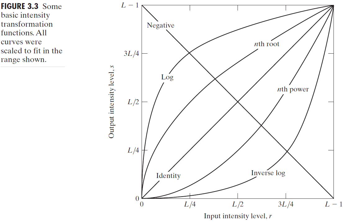
3.2 Some Basic Intensity Transformation Functions

3.2.1 Image Negatives

$$
s=L-1-r
$$

3.2.2 Log Transformations

$$
s = c log (1 + r)
$$

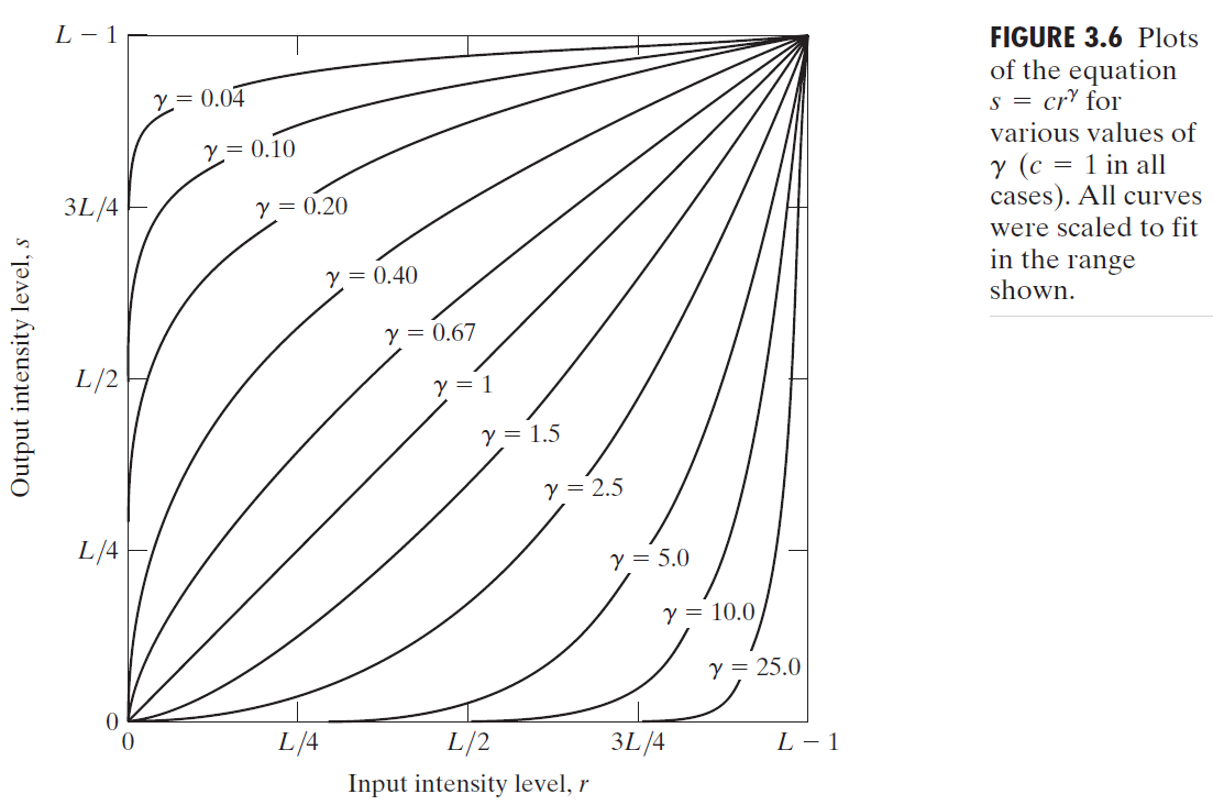
3.2.3 Power-Law (Gamma) Transformations

$$
s=cr^\gamma
$$

A variety of devices used for image capture, printing, and display respond
according to a power law. The process used to correct these power-law response phenomena is called gamma correction.

Trying to reproduce colors accurately also requires some knowledge of gamma correction because varying the value of gamma changes not only the intensity, but also the ratios of red to green to blue in a color image.

In addition to gamma correction, power-law transformations are useful for
general-purpose contrast manipulation.

3.2.4 Piecewise-Linear Transformation Functions

Contrast stretching

Contrast stretching is a process that expands the range of intensity levels in an image so that it spans the full intensity range of the recording medium or display device

Intensity-level slicing

Highlighting a specific range of intensities in an image.

Bit-plane slicing

Pixels are digital numbers composed of bits. Instead of highlighting intensity-level ranges, we could highlight the contribution made to total image appearance by specific bits.

Decomposing an image into its bit planes is useful for analyzing the rela
tive importance of each bit in the image.

Also, this type of decomposition is useful for image compression.

3.3 Histogram Processing

The histogram of a digital image with intensity levels in the range $[0,L-1]$ is a discrete function:
$$
h(r_k)=n_k
$$

where $r_k$ is the $k$th intensity value and $n_k$ is the number of pixels in the image with intensity $r_k$.

It is common practice to normalize a histogram by dividing each of its components by the total number of pixels in the image. Thus, a normalized histogram is given by
$$
p(r_k)=r_k/MN
$$
An image with low contrast has a narrow histogram located typically
toward the middle of the intensity scale. The components of the histogram in the high-contrast image cover a wide range of the intensity scale and that the distribution of pixels is not too far from uniform.

3.3.1 Histogram Equalization

we focus attention on transformations of the form
$$
s=T(r)\ ,\ 0\le r\le L-1
$$

$T(r)$ is a monotonically increasing function in the interval $0\le r\le L-1$
$0 \le s\le L-1$ for $0\le r\le L-1$

Let $p_r(r)$ and $p_s(s)$ denote the PDFs of $r$ and $s$, respectively. The PDF of the transformed (mapped) variable s can be obtained using the simple formula:
$$
p_s(s)=p_r(r)|\frac{dr}{ds}|
$$
Let the transformation function be the cumulative distribution function (CDF):
$$
s=T(r)=(L-1)\int^r_0p_r(w)dw
$$
To find the $p_s(s)$ corresponding to the transformation, we use Eq.(9):
$$
\frac{ds}{dr} =\frac{dT(r)}{dr}=(L-1)\frac{d}{dr}[\int^r_0p_r(w)dw]=(L-1)p_r(r)
$$

$$
p_s(s)=p_r(r)|\frac{dr}{ds}|=p_r(r)|\frac{1}{(L-1)p_r(r)}|=\frac{1}{L-1}
$$

It is important to note the resulting $p_s(s)$ always is uniform, independently of the form of $p_r(r)$ .

The transformation (mapping) $T(r_k)$ in this equation is called a histogram equalization or histogram linearization transformation.

3.3.2 Histogram Matching (Specification)

The method used to generate a processed image that has a specified histogram is called histogram matching or histogram specification.

an image whose intensity levels have a specified probability density function can be obtained from a given image by using the following procedure:

Obtain $p_r(r)$ from the input image and use Eq. (10) to obtain the values of $s$.
Use the specified PDF to obtain the transformation function $G(z)$.
Obtain the inverse transformation $z=G^{-1}(s)$
Obtain the output image by Eq. (10)

3.3.3 Local Histogram Processing

The procedure is to define a neighborhood and move its center from pixel to pixel. At each location, the histogram of the points in the neighborhood is computed and either a histogram equalization or histogram specification transformation function is obtained.

As often is the case with histogram equalization of smooth, noisy regions, this image shows significant enhancement of the noise

3.3.4 Using Histogram Statistics for Image Enhancement

The mean is a measure of average intensity, the variance (or standard deviation) is a measure of contrast in an image.

When working with only the mean and variance, it is common practice to estimate them directly from the sample values, without computing the histogram.

3.4 Fundamentals of Spatial Filtering

We focus attention first on linear filters and then illustrate some
simple nonlinear filters.

There is a one-to-one correspondence between linear spatial filters and filters in the frequency domain.

3.4.2 Spatial Correlation and Convolution

correlation
$$
w(x,y)☆f(x,y)=\sum^a_{s=-a}\sum^b_{t=-b}w(s,t)f(x+s,y+t)
$$

convolution
$$
w(x,y)★f(x,y)=\sum^a_{s=-a}\sum^b_{t=-b}w(s,t)f(x-s,y-t)
$$

It should be point out that you are likely to encounter the terms, convolution filter, convolution mask or convolution kernel. As a rule, these terms are used to denote a spatial filter, and not necessarily that the filter will be used for true convolution.

3.4.3 Vector Representation of Linear Filtering

$$
R=\sum^{mn}_{k=1}w_kz_k=\mathbf{w}^T\mathbf{z}
$$

3.4.4 Generating Spatial Filter Masks

All we can do with linear filtering is to implement a sum of products.

3.5 Smoothing Spatial Filters

Smoothing filters are used for blurring and for noise reduction.

3.5.1 Smoothing Linear Filters

averaging filters (lowpass filters): linear spatial filter is simply the average of the pixels contained in the neighborhood of the filter mask.
box filter: A spatial averaging filter in which all coefficients are equal.
weighted average: pixels are multiplied by different coefficients, thus giving more importance (weight) to some pixels at the expense of others.

3.5.2 Order-Statistic (Nonlinear) Filters

Order-statistic filters are nonlinear spatial filters whose response is based on ordering (ranking) the pixels, and then replacing the value of the center pixel with the value determined by the ranking result.

Median filters are particularly effective in the presence of impulse noise.

median filter: replaces the value of a pixel by the median of the intensity
values in the neighborhood of that pixel
impulse noise (salt-and-pepper noise), its appearance as white and black dots superimposed on an image

3.6 Sharpening Spatial Filters

The principal objective of sharpening is to highlight transitions in intensity.

Because averaging is analogous to integration, it is logical to conclude that sharpening can be accomplished by spatial differentiation.

Image differentiation enhances edges and other discontinuities (such as noise) and deemphasizes areas with slowly varying intensities.

3.6.1 Foundation

The second derivative enhances fine detail much better than the first derivative and are much easier to implement than first derivates, so we focus our attention initially on second derivatives.

3.6.2 Using the Second Derivative for Image Sharpening—The Laplacian

isotropic filters: response is independent of the direction of the discontinuities in the image. rotation invariant.

The simplest isotropic derivative operator is the Laplacian:
$$
\nabla^2f=\frac{\partial^2f}{\partial x^2}+\frac{\partial^2f}{\partial y^2}\
=f(x+1,y)+f(x-1,y)+f(x,y+1)+f(x,y-1)-4f(x,y)
$$

the Laplacian is a linear operator
The diagonal directions can be incorporated in the definition of the digital Laplacian by adding two more terms to Eq. (16)
implementations of the Laplacian with reverse signs found frequently in practice.

The basic way in which we use the Laplacian for image sharpening is
$$
g(x,y)=f(x,y)+c[\nabla^2f(x,y)]
$$

3.6.3 Unsharp Masking and Highboost Filtering

unsharp masking :

Blur the original image.
Subtract the blurred image from the original (the resulting difference is
called the mask.)
Add a weighted portion($k$) of the mask back to the original image.

When $k=1$, we have unsharp masking, as defined above.

When $k>1$, the process is referred to as highboost filtering.

Choosing $k<1$, de-emphasizes the contribution of the unsharp mask.

3.6.4 Using First-Order Derivatives for (Nonlinear) Image Sharpening—The Gradient

For a function $f(x,y)$, the gradient of $f$ at coordinates $(x, y)$ is defined as the two-dimensional column vector
$$
\nabla f=grad(f)=\begin{bmatrix} g_x\ g_y \end{bmatrix}=\begin{bmatrix} \frac{\partial f}{\partial x}\ \frac{\partial f}{\partial y} \end{bmatrix}
$$

This vector has the important geometrical property that it points in the direction of the greatest rate of change of $f$ at location $(x, y)$.

The magnitude (length) of vector $\nabla f$, denoted as $M(x, y)$, where
$$
M(x,y)=mag(\nabla f)=\sqrt{g_x^2+g_y^2}
$$

is the value at $(x, y)$ of the rate of change in the direction of the gradient vector.

It is common practice to refer to this image as the gradient image

The magnitude of this vector is not linear operators, and the partial derivatives are not rotation invariant, so, in some implementations, it is more suitable computationally to approximate the squares and square root operations by absolute values:
$$
M(x,y)\approx |g_x|+|g_y|
$$

This expression still preserves the relative changes in intensity, but the isotropic property is lost in general

3.8 Using Fuzzy Techniques for Intensity Transformations and Spatial Filtering

3.8.2 Principles of Fuzzy Set Theory

a fuzzy set is an ordered pair consisting of values of z and a corresponding membership function that assigns a grade of membership to each z.That is
$$
A={z,\mu_A(z)|z\in Z}
$$

all $z$s for which $\mu_A(z)=1$ are full members of the set, all $z$s for which $\mu_A(z)=0$ are not members of the set, and all $z$s for which $\mu_A(z)$ is between 0 and 1 have partial membership in the set

3.8.3 Using Fuzzy Sets

defuzzification: One of the approaches used most frequently is to compute the center of gravity of this set

We can use the preceding material to summarize the principal steps followed in the application of rule-based fuzzy logic:

Fuzzify the inputs
Perform any required fuzzy logical operations
Apply an implication method
Apply an aggregation method to the fuzzy sets from step 3
Defuzzify the final output fuzzy set